Decoding the Graph-Wall-Tome Connection
An important aspect of the prompt is that neither the Graph, nor the Wall or the Tome are that important on their own. Only together does their explanatory power exceed the limits of any part alone. The common threads that run through all of them are what matter: what is common among them is what should be expanded, and what is particular to one should be promoted and developed if it is a part of fundamental physics toolkit, or removed if it isn't.
| Graph-Wall-Tome Connection | |

| |
| Information | |
|---|---|
| Topic | Graph, Wall, Tome |
| Leader | Aardvark |
| Start Date | 21 April 2020 |
| New Graph-Wall Mind Map | Link |
| Graph Mind Map | Link |
| Google Drive | Drive |
| Master Planning | Doc |
| Links | |
| Website | Homepage |
| Discord | Invite |
| All Projects | |
The goals of this project are to:
- Identify the common threads (the "unifying idea") in the Graph, Wall, and Tome. These will indicate how to Edit the Graph and Deface the Wall.
- Create and collect resources that make it easy to understand them, thus contributing to Rewriting the Tome.
Guiding Questions and Comments by Eric Weinstein
$$F_A$$ is the curvature tensor associated with the connection or vector potential $$A$$.
$$R$$ is a scalar value, describing the "curvature of the spacetime manifold" at each point along the manifold. It's based on a concept of 'parallel transport', where you move a vector around some path on the manifold.
$$R$$ can be computed at each point on the manifold, and describes the difference in the vector's angle after following an infinitesimally small path around the neighborhood of that point, vs. what it was originally. The video does a great job of visualizing when and why that vector angle change would happen, with flat vs. curved manifolds.
In the video, they focus first on the curvature of space. Hopefully they incorporate back in curvature in time, because that's less obvious.
The same video then proceeds to explain $$R_{\mu v}$$. It progresses through some concepts.
Computing length in non-orthogonal bases
First, just describing the length of a vector on a curved space is hard. It is given by:
$$Length^{squared} = g_{11}dX^{1}dX^{1} + g_{12}dX^{1}dX^{2} + g_{21}dX^{2}dX^{1} + g_{22}dX^{2}dX^{2}$$
Some notes:
- This is not Pythagorean theorem, because $$dX^{1}$$ and $$dX^{2}$$ are not perpendicular.
- Instead, looks like a formula to get the diagonal from two opposite vertices in a parallelogram.
- If $$dX^{1}$$ and $$dX^{2}$$ are perpendicular, then $$g_{12}$$ and $$g_{21}$$ would be 0, and we would get $$Length^{squared} = g_{11}(dX^{1})^{2} + g_{22}(dX^{2})^{2}$$
- See: the video @ 14m27s
Computing vector rotation due to parallel transport
Then, they show parallel transport when following a parallelogram, but over a curved 3D manifold. To compute the vector rotation by components, they show:
$$dV^{1} = dX^{1}dX^{2} (V^{1}R^{1}_{112} + V^{2}R^{1}_{212} + V^{3}R^{1}_{312})$$
$$dV^{2} = dX^{1}dX^{2} (V^{1}R^{2}_{112} + V^{2}R^{2}_{212} + V^{3}R^{2}_{312})$$
$$dV^{3} = dX^{1}dX^{2} (V^{1}R^{3}_{112} + V^{2}R^{3}_{212} + V^{3}R^{3}_{312})$$
or, using $$i$$ to summarize across all 3 components (difference vectors):
$$dV^{i} = dX^{1}dX^{2} (V^{1}R^{i}_{112} + V^{2}R^{i}_{212} + V^{3}R^{i}_{312})$$
or , using $$j$$ to index over all 3 components (original vector):
$$dV^{i} = dX^{1}dX^{2} \Sigma_{j} [(V^{j}R^{i}_{j12}]$$
See: the video @ 19m33s
Open questions:
- Why a parallelogram?
- How to properly overlay the parallelogram onto the 3d manifold, in order to do the parallel transport?
- How does this relate to the length computation above?
Putting it all together
Now, moving to 4D, we can compute $$R_{\mu v}$$ as:
$$R_{00} = R^{0}_{000} + R^{1}_{010} + R^{2}_{020} + R^{3}_{030}$$
$$R_{10} = R^{0}_{100} + R^{1}_{110} + R^{2}_{120} + R^{3}_{130}$$
$$R_{01} = R^{0}_{001} + R^{1}_{011} + R^{2}_{021} + R^{3}_{030}$$
etc.
Indexing i over all 4 component vectors / dimensions, we get:
$$R_{00} = \Sigma_{i} R^{i}_{0i0}$$
$$R_{10} = \Sigma_{i} R^{i}_{1i0}$$
$$R_{01} = \Sigma_{i} R^{i}_{0i1}$$
etc.
Summarizing on $$\mu$$, we get:
$$R_{\mu 0} = \Sigma_{i} R^{i}_{\mu i0}$$
$$R_{\mu 1} = \Sigma_{i} R^{i}_{\mu i1}$$
etc
Summarizing on $$v$$, we get:
$$R_{\mu v} = \Sigma_{i} R^{i}_{\mu iv}$$
Open questions:
- If we hadn't moved from 3D to 4D, what would this all have looked like?
- What does this have to do with the parallelogram?
- Why are there two indices?
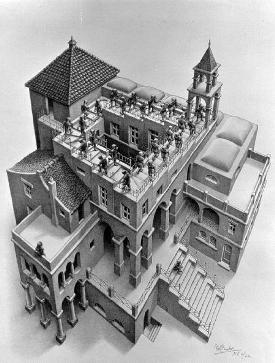
We’ve heard Eric talk about Penrose stairs and spinors - essentially phenomena where you cannot return to the original state through a 360 degree rotation, but require a 720 degree rotation.
From theplebistocrat:
Generally, we're wanting to understand how fermions arise from - or are embedded within / upon - topological "spaces" that have distinct rules which govern operations within those topological spaces, and then how those rules produce higher dimensional operations in corresponding spaces.
Just intuitively, and geometrically speaking, the image that I'm getting when describing all of this and trying to hold it in my head is the image of a sort of Penrose Tower of Babel, where the fundamental underlying structures reach upwards (but also downwards and inwards?) before reaching a critical rotation that corresponds to a collapse of structure into a higher dimensional fiber bundle.
But doesn't this require the symmetry break? How is left and right rotation in a subspace transformed into verticality? This is a crazy rabbit hole, friends. Keep your chins up. Let me know if this was helpful or leading astray.
"The source code of the universe is overwhelmingly likely to determine a purely geometric operating system written in a uniform programming language." - Eric Weinstein
- Another valuable resource is the comments Eric made regarding how the Wall should be modified.
Direct Connections between the Graph, the Wall, and the Tome
Connections between the Graph and the Wall
An interactive version of the Wall that shows direct connections to the graph is available here.
Connections between the Wall and the Tome
Connections between the Graph and the Tome